Udacity Machine Learning Nanodegree
Bank Marketing Campaign Predictive Analysis
Sai Charan Adurthi
December 4th, 2018
I. Definition
Banks collect huge records of information about their customers. This data can be used to create and keep clear relationship and connection with the customers in order to target them individually for specific products or banking offers. Usually, the selected customers are contacted via: personal contact, telephone, cellular, mail, email and any other contacts to advertise the new product/service or propose an offer. This type of marketing is known as direct marketing. In fact, direct marketing is in the main a strategy of many of the banks and insurance companies for interacting with their customers.
Historically, the name and identification of the term direct marketing was first suggested in 1967 by Lester Wunderman, which is why he is considered as the father of direct marketing.
In addition, some of the banks and financial-services companies may depend only on strategy of mass marketing for promoting a new service or product to their customers. In this strategy, a single communication message is broadcasted to all customers through media such as television, radio or advertising firm, etc... In this approach, companies do not set up a direct relationship to their customers for new-product offers. In fact, many of the customers are not interested or just don't respond to this kind of sales promotion.
Accordingly, banks, financial-services companies and other companies are shifting away from mass marketing strategy because of its ineffectiveness, and they are now targeting most of their customers by direct marketing for specific product and service offers.
Due to the positive results clearly measured; many marketers attractive to the direct marketing. For example, if a marketer sends out 1,000 offers by mail and 100 respond to the promotion, the marketer can say with confidence that the campaign led immediately to 10% direct responses.
This metric is known as the 'Response Rate', and it is one of many clear quantifiable success metrics employed by direct marketers.
Direct marketing is becoming a very important application in data mining these days. It is used widely in direct marketing to identify prospective customers for new products, by using purchasing data, a predictive model to measure that a customer is going to respond to the promotion or an offer. Data mining has gained popularity for illustrative and predictive applications in banking processes.
Problem Statement
All bank marketing campaigns are dependent on customers data. The size of these data sources make it impossible for a human analyst to extract interesting information that helps in the decision-making process. Data mining models help us achieve this.
The purpose is to increase the campaign effectiveness by identifying significant characteristics that affect the success (the deposit subscribed by the client) based on a handful of algorithms that we will test (e.g. Logistic Regression, Gaussian Naive Bayes, Decision Trees and others). The experiments will demonstrate the performance of models by statistical metrics like accuracy, sensitivity, precision, recall, etc..
Metrics
The evaluation metrics proposed are appropriate given the context of the data, the problem statement, and the intended solution. The performance of each classification model is evaluated using three statistical measures; classification accuracy, sensitivity and specificity. It is using true positive (TP), true negative (TN), false positive (FP) and false negative (FN). The percentage of Correct/Incorrect classification is the difference between the actual and predicted values of variables. True Positive (TP) is the number of correct predictions that an instance is true, or in other words; it is occurring when the positive prediction of the classifier coincided with a positive prediction of target attribute. True Negative (TN) is presenting a number of correct predictions that an instance is false, (i.e.) it occurs when both the classifier, and the target attribute suggests the absence of a positive prediction. The False Positive (FP) is the number of incorrect predictions that an instance is true. Finally, False Negative (FN) is the number of incorrect predictions that an instance is false. Table below shows the confusion matrix for a two-class classifier.
Predicted No | Predicted Yes | |
Actual No | TN | FN |
Actual Yes | FP | TP |
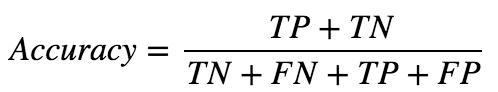
Classification accuracy is defined as the ratio of the number of correctly classified cases and is equal to the sum of TP and TN divided by the total number of cases (TN + FN + TP + FP).
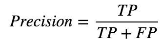
Precision is defined as the number of true positives (TP) over the number of true positives plus the number of false positives (FP).
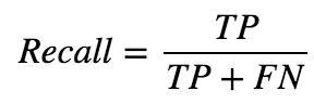
Recall is defined as the number of true positives (TP) over the number of true positives plus the number of false negatives (FN).
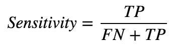
Sensitivity refers to the rate of correctly classified positive and is equal to TP divided by the sum of TP and FN.
Sensitivity may be referred as a True Positive Rate.
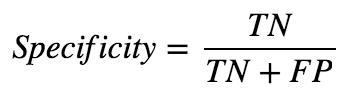
Specificity refers to the rate of correctly classified negative and is equal to the ratio of TN to the sum of TN and FP
II. Analysis
Data Exploration
The data is related with direct marketing campaigns of a Portuguese banking institution. The marketing campaigns are based on phone calls. Often, more than one contact to the same client was required, in order to check if the product (bank term deposit) would be ('yes') or not ('no') subscribed. The classification goal is to predict if the client will subscribe (yes/no) a term deposit (variable y).
Input variables:
Exploratory Visualization
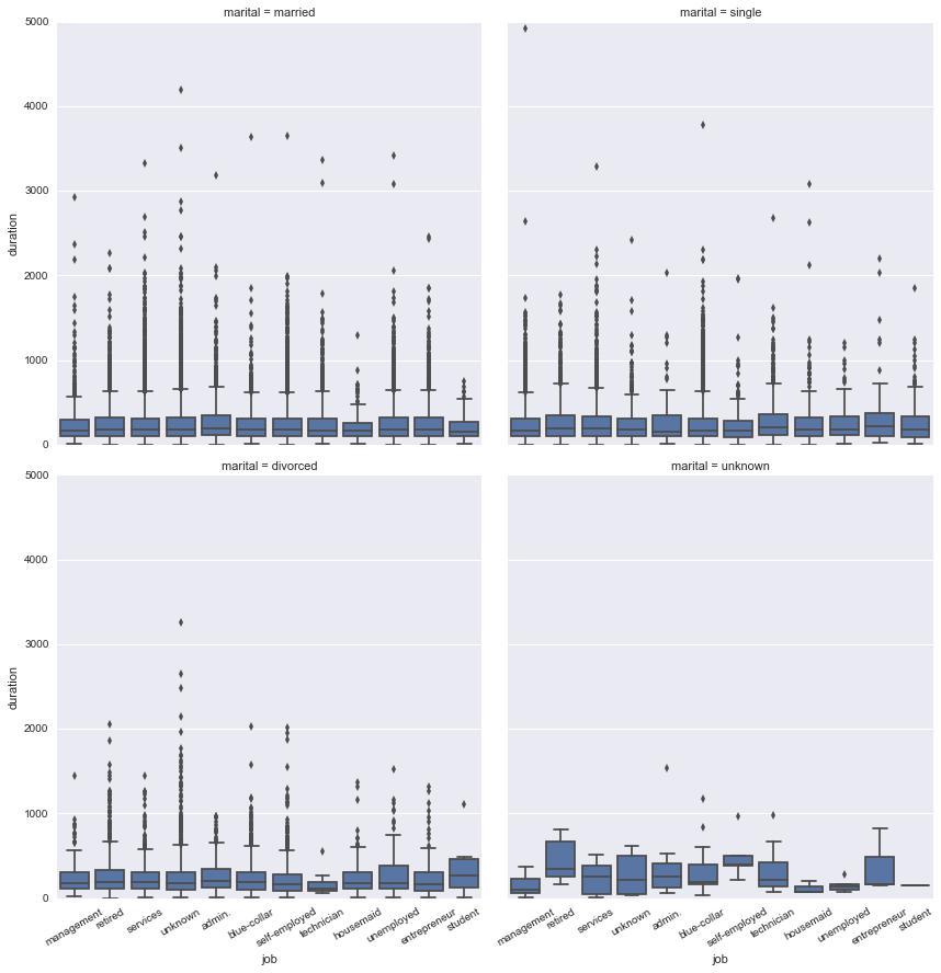
Fig. 1 shows data distribution of `job` factors with `duration` and split by `marital` status. It is hard to spot relevances between factors from this plot. We can pick few numeric variables and plot them to see if we can find any different patterns.
Fig. 1 Job vs duration split by marital status
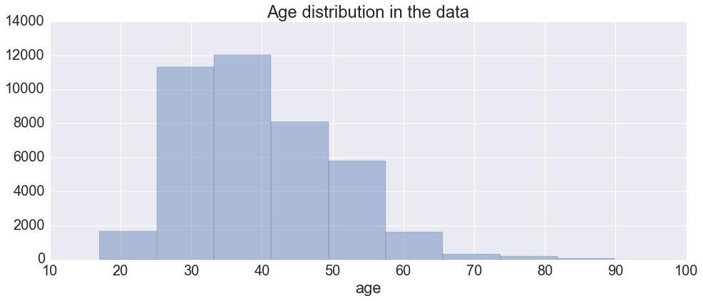
Fig.2 shows age distribution in the data and is a normal distribution with slight left skewness. This shows that majority of the responses are in 25-40 age group.
Fig 2. Age distribution
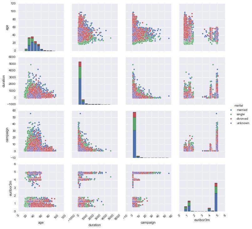
Fig. 3 Scatterplot matrix of `age`, `duration`, `campaign` and `euribor3m`
We can see some interesting patterns in Fig. 3, there are splits in data for `euribor3m` and also note that the durations are smaller for age > 60 and other such relevant information. We could also check data distributions of each variable but I will leave it out for now and move ahead.
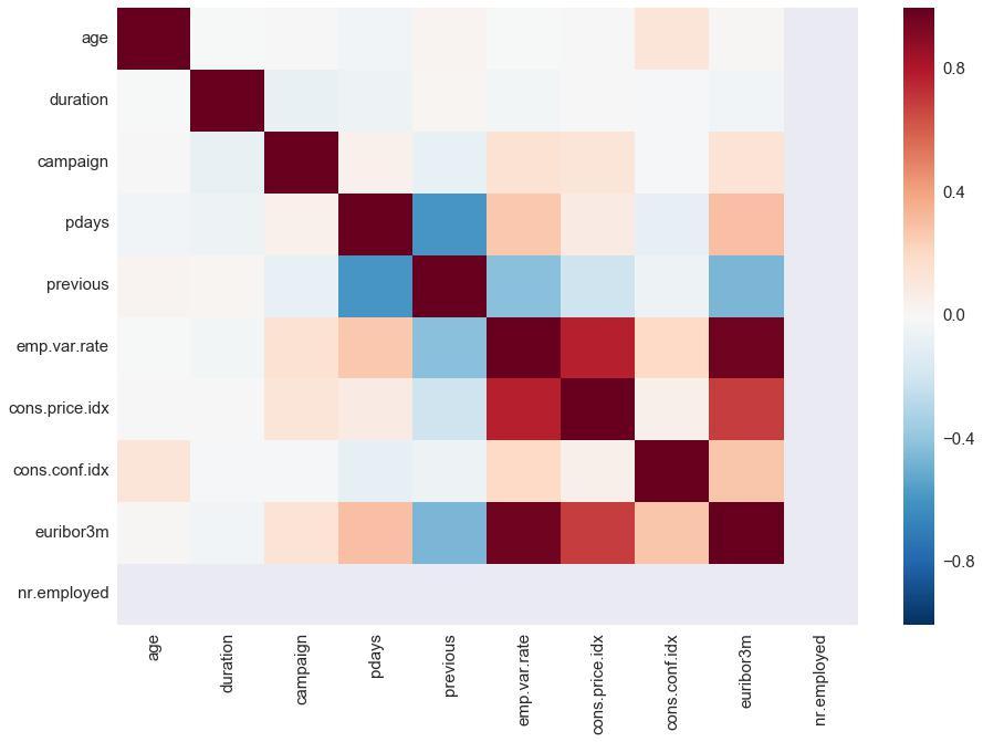
We apply scatterplot matrix on whole dataset to visualize inherent relationships between variables in the data shown in Fig. 4. But we can conclude that there isn't a strong relationship
Fig. 4 Scatterplot matrix
Algorithms and Techniques
The given dataset is a typical supervised learning problem for which tree type models perform a lot better than the rest. We don't know which algorithms would be fit for this problem or what configurations to use.
So, let's pick few algorithms to evaluate.
We are using 5-fold cross validation to estimate accuracy. This will split our dataset 5 parts, train on 4 and test on 1 and repeat for all combinations of train-test splits. Also, we are using the metric of accuracy to evaluate models. This is a ratio of the number of correctly predicted instances in divided by the total number of instances in the dataset multiplied by 100 to give a percentage (e.g. 95% accurate). We will be using the scoring variable when we run build and evaluate each model next.
Benchmark Model
Below table highlights performances of various models that were tried with their accuracies and errors. The standard Extreme Gradient Boosting (XGB) model with default parameters yields 91.4% accuracy on training data. So will consider it as benchmark and try to beat the benchmark with hyperparameter tuning.
Algorithms | Accuracy | Std. Error |
Logistic Regression | 0.909611 | 0.005315 |
CART | 0.888800 | 0.005325 |
Random Forest | 0.912525 | 0.006937 |
AdaBoost | 0.913218 | 0.007852 |
XGBoost | 0.914640 | 0.007852 |
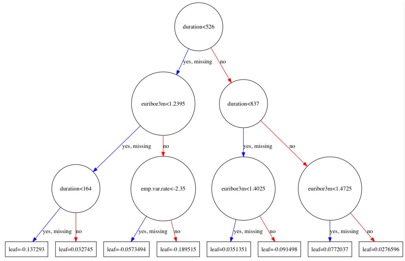
Fig. 5 Decision Tree
III. Methodology
Data Preprocessing
We will prepare the data by splitting feature and target/label columns and also check for quality of given data and perform data cleaning. To check if the model I created is any good, I will split the data into `training` and `validation` sets to check the accuracy of the best model. We will split the given `training` data in two ,70% of which will be used to train our models and 30% we will hold back as a `validation` set.
There are several non-numeric columns that need to be converted. Many of them are simply yes/no, e.g. housing. These can be reasonably converted into 1/0 (binary) values. Other columns, like profession and marital, have more than two values, and are known as categorical variables. The recommended way to handle such a column is to create as many columns as possible values (e.g. profession_admin, profession_blue-collar, etc.), and assign a 1 to one of them and 0 to all others. These generated columns are sometimes called dummy variables, and we will use the pandas.get_dummies() function to perform this transformation.
Several Data preprocessing steps like preprocessing feature columns, identifying feature and target columns, data cleaning and creating training and validation data splits were followed and can be referenced for details in attached jupyter notebook.
Implementation
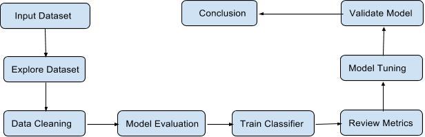
The project follows typical predictive analytics hierarchy as shown below:
Refinement
We will prepare the data by splitting feature and target/label columns and also check for quality of given data and perform data cleaning. To check if the model we created is any good, we will split the data into training and validation sets to check the accuracy of the best model. We will split the given training data in two ,70% of which will be used to train our models and 30% we will hold back as a validation set.
We performed hyper tuning of parameters of XGBoost wrapper from scikit-learn library and the parameters tuned were shown in below table:
Parameter | Description | Values Tested | Best Value | |||
max_depth | maximum depth of a tree to | 5 | ||||
(3,4,5,6,7,8,9) | ||||||
control overfitting | ||||||
min_child_weight | minimum sum of weights of all | 3 | ||||
(2,3,4,5,6,7) | ||||||
observations required in a | ||||||
child | ||||||
gamma | minimum loss reduction | (0,0.1,0.2,0.3,0.4,0. | 0.1 | |||
required to make a split | 5,0.6,0.7,0.9,1.0) | |||||
reg_alpha | L1 regularization term on | (0,2,4) | 2 | |||
weights | ||||||
reg_lambda | L2 regularization term on | (1,3,5 | 5 | |||
weights | ||||||
subsample | Subsample ratio of the | (0.5,1.0) | 1 | |||
training instance | ||||||
colsample_bytree | Subsample ratio of columns | (0.5,1.0) | 1 | |||
when constructing each tree | ||||||
colsample_bylevel | Subsample ratio of columns | (0.5,1.0) | 1 | |||
for each split, in each level | ||||||
IV. Results
Model Evaluation and Validation
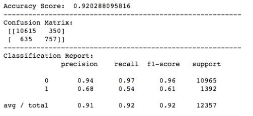
A final model with above list of tuned parameters is generated. The output of this tuned model came just about 0.2% higher in accuracy vs the untuned model.
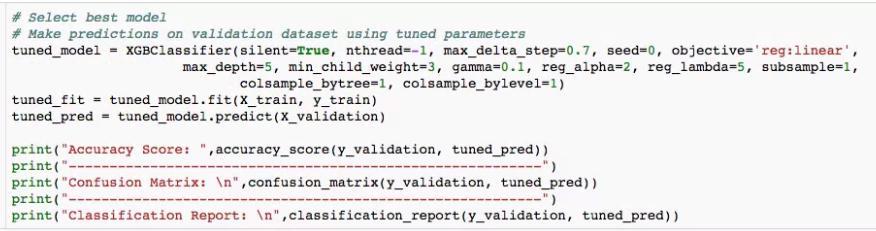
Code snippet of final model is shown below:
Justification
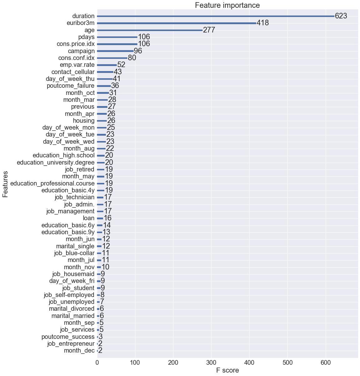
There is room for improvement on the final results, the tuned final model made no significant improvement over the untuned model. There could be more ways we could improve the score, particularly by selecting a subset of features using the ranking obtained from observing feature importance ranking and then performing the same exercise we did as described above. But this would be out of scope of this report for now.
Benchmark Model | Final Model | |
(Untuned XGBClassifier Model) | (Tuned XGBClassifier Model) | |
Accuracy Score | 0.9184 | 0.9202 |
V. Conclusion
Free-Form Visualization
The importance of each feature was visualized with the following plot:
Reflection
The most important and time consuming part of the problem was data cleansing and processing as there were multiple columns with null values. Once the data was prepared and ready, the next challenge was to pick an algorithm that could be best suited for the problem we choose to solve. With experience and prior knowledge and also the outcome of accuracy on training data, we observed that XGBoost performed the best out of others.
Improvements
We chose to use untuned XGBoost and benchmark it with tuned XGBoost model. We implemented the tuning using XGBoost’s easy to use scikit-learn wrapper. The parameters were tuned using GridSearchCV. To our surprise the tuned model did not show any improve over the untuned model.